Le 29 octobre dernier, la version 4.7.2 de Sage est sortie. C'est dans cette version de Sage (merci beaucoup à Rob Beezer qui a arbitré cette contribution) qu'a été ajouté le code que j'ai écrit en juin dernier pour résoudre le puzzle appelé Quantumino. Ce puzzle avait été laissé à la salle à manger du Laboratoire de Combinatoire Informatique Mathematique de Montréal par Franco Saliola durant l'hiver 2011...

• Puzzle Quantumino par Family Games America
• Quantumino sur Youtube

La solution utilise le code des liens dansants qui se trouvait déjà dans Sage pour résoudre le problème du Sudoku. Les liens dansants ont été introduits par Donald Knuth en 2000 pour résoudre le pavage d'une région 2D par des pentaminos. Ici nous utilisons la même méthode en dimension quelconque et nous l'appliquons pour résoudre le puzzle Quantumino. Voici les deux pages concernées de la documentation de Sage:

• Tiling Solver
• Quantumino Solver

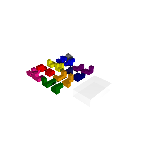
Voici les 17 blocs de bois du puzzle Quantumino:

sage: from sage.games.quantumino import show_pentaminos
sage: show_pentaminos()

Pour résoudre le puzzle où le pentamino numéroté 7 est mis de côté:

sage: from sage.games.quantumino import QuantuminoSolver
sage: s = QuantuminoSolver(7).solve().next()
sage: s.show3d().show(frame=False)

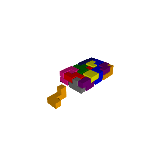
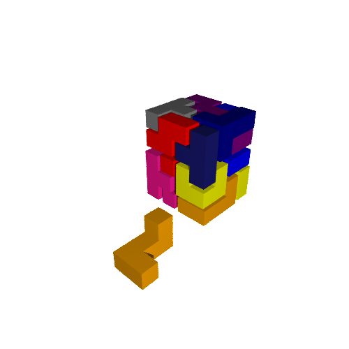
Pour obtenir d'autres solutions, utilisez l'itérateur retourné par la fonction solve. Notez que trouver la première solution est plus long car on a besoin de créer les données complètes pour décrire le problème:

sage: it = QuantuminoSolver(7).solve()
sage: 1st_solution = it.next()
sage: 2nd_solution = it.next()
sage: 3rd_solution = it.next()
sage: 3rd_solution.show3d().show(frame=False)

Pour obtenir la solution à l'intérieur d'autres boîtes:

sage: s = QuantuminoSolver(7, box=(4,4,5)).solve().next()
sage: s.show3d()

S'il n'y a pas de solution, l'itération se termine immédiatement:

sage: QuantuminoSolver(7, box=(3,3,3)).solve().next()
Traceback (most recent call last):
...
StopIteration

Si vous êtes patients, vous pouvez essayer de calculer le nombre de solutions. Attention, il y en a beaucoup!:

sage: from sage.games.quantumino import QuantuminoSolver
sage: q = QuantuminoSolver(7)
sage: q.number_of_solutions()   # prendra plusieurs jours de calculs

Le code permet aussi l'introspection. À partir d'un objet de la classe sage.combinat.tiling.TilingSolver, il est possible de récupérer les lignes de la matrice décrivant le problème de couverture exacte en question. Il est également possible d'obtenir une instance du solveur DLX et de tester certaines choses:

sage: q = QuantuminoSolver(0)
sage: T = q.tiling_solver()
sage: T
Tiling solver of 16 pieces into the box (5, 8, 2)
Rotation allowed: True
Reflection allowed: False
Reusing pieces allowed: False
sage: rows = T.rows()
sage: len(rows)
5484
sage: x = T.dlx_solver()
sage: x
<sage.combinat.matrices.dancing_links.dancing_linksWrapper object at ...>

Lorsque j'ai participé aux Sage Days 31 à Seattle en juin dernier (conférence dont l'objectif était de développer le Sage Notebook), j'ai rencontré Jason Grout (Drake University, Iowa). Le projet de Jason était de parvenir à utiliser Sage directement dans une page web (voir la discussion public single cell sur sage-devel pour en savoir plus).

Son projet est toujours en cours, mais il semble déjà être fonctionnel à en juger la page web de Rob Beezer (University of Puget Sound, Washington) qui illustre un exemple en faisant des calculs sur le graphe de Petersen et le calcul d'un factoriel.

Essayons d'immiter ce qu'il a fait! Dans la cellule qui suit, on définit une fonction de deux variables \(f(x,y) = \frac{xy}{e^{x^2 + y^2}}\) et on affiche ses lignes de niveau. Cliquez sur le bouton Calculer pour les afficher. Vous pouvez aussi changer la fonction et réévaluer la cellule.

Les graphes 3D fonctionnent aussi. Par exemple, ajoutez la ligne suivante dans la cellule et cliquez sur Calculer:

plot3d(f, (x,-4,4), (y,-4,4))

Vous obtiendrez le graphe 3D de la surface \(z = f(x,y)\).

<!-- Sage Free Trial  -->
<script type="text/javascript" src="http://aleph.sagemath.org/static/jquery.min.js"></script>
<script type="text/javascript" src="http://aleph.sagemath.org/embedded_sagecell.js"></script>
<script>
$(function() {
var makecells = function() {
singlecell.makeSagecell({
inputLocation: '#first_cell',
editor: 'codemirror',
replaceOutput: true,
hide: ['editorToggle', 'sageMode', 'computationID', 'messages', 'sessionTitle', 'done', 'sessionFilesTitle', 'sessionFiles',  'files', 'sageMode'],
evalButtonText: 'Calculer'
});
}
sagecell.init(makecells);
})
</script>

<!-- First cell -->
<div id="first_cell"><script type="text/code">f(x,y) = x * y / exp(x^2 + y^2)
G = implicit_plot(f(x,y) , (x,-3,3), (y,-3,3), contours=30, cmap='hsv')
G.show(aspect_ratio=1)
</script></div>

Il existe une méthode peu connue pour connaître les composantes de Sage utilisées par un calcul. Supposons qu'on a le calcul suivant:

sage: g = Permutation('(2,3)')
sage: h = Permutation('(2,3,4,5)')
sage: S = PermutationGroup([g, h])
sage: c = S.conjugacy_classes_subgroups()

Pour connaître les systèmes utilisés par le calcul précédent, on écrit:

sage: import sage.misc.citation
sage: sage.misc.citation.get_systems('S.conjugacy_classes_subgroups()')
['GAP']

Cela permet de savoir par exemple quels systèmes on doit citer dans un article de recherche qui les utilise. Voici un autre exemple qui montre que quatre systèmes sont utilisés pour calculer l'intégrale \(\int \cos(x^2) dx\):

sage: from sage.misc.citation import get_systems
sage: get_systems("integrate(cos(x^2), x)")
['MPFI', 'ginac', 'GMP', 'Maxima']

L'existence de la fonction get_systems a été rappelée en juillet 2011 par Mike Hansen dans cette conversation sur sage-devel : Citing used Sage components automatically.

In Sage, we can create 3d graphic objects like the following:

sage: a = line3d([(0,1,0), (0,0,0), (1,0,0), (2,0,0)], radius=0.1)
sage: b = line3d([(1,0,0), (1,0.5,0)], radius=0.1)
sage: g = a + b

sage: x,y = map(vector, g.bounding_box())
sage: g.frame_aspect_ratio(tuple(y-x))      # this sets the aspect ratio to 1

sage: g

Rotate the graphic object until you get a view you like.

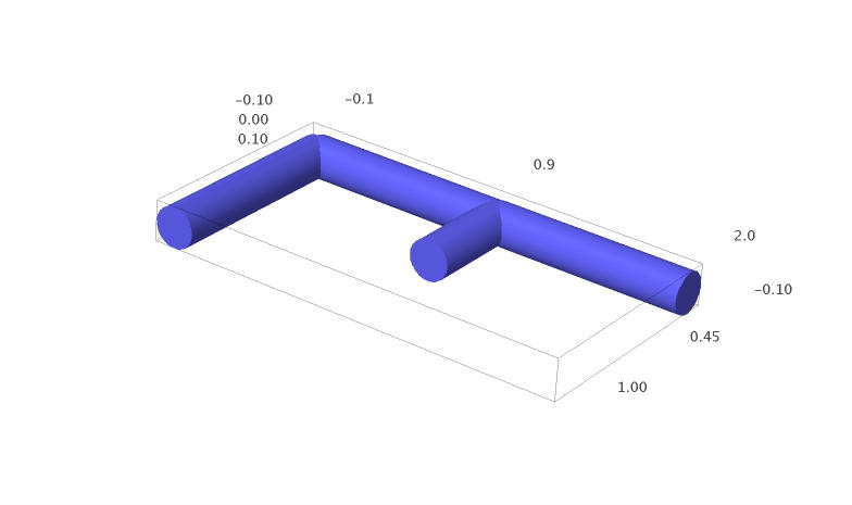
One can save an image as a jpg, but the quality is not always good and one could prefer to draw the image using another tool like tikz code. But how to draw the 3d graphic object with the same projection?

To get information about the actual view and hopefully about the camera position, right clic on the image and go to the current state ("État courant" in French).

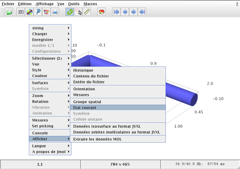
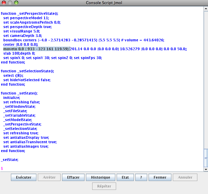
In the window that pops up, the information you need is the line starting with:

moveto 0.0 {933 -323 161 119.59}

According to the Jmol documentation of the moveto method (and also after doing some moveto tests in the script window), I understand that this tells that a rotation of angle \(119.59\) degrees is done on the axis \((933, -323, 161)\). The rotation is done counterclockwise (right-hand rule). From this information, we may then compute the rotation matrix using rotate_arbitrary method written by Robert Bradshaw and available in Sage. Note that the rotation of the method rotate_arbitrary is done counterclockwise (left-hand rule).

sage: from sage.plot.plot3d.transform import rotate_arbitrary
sage: v = (933, -323, 161)
sage: angle = 119.59                    # righ-hand rule
sage: angle = - angle                   # left-hand rule
sage: angle_rad = angle * pi / 180
sage: M = rotate_arbitrary(v, angle_rad)
sage: M
[  0.805577517225  -0.589785522899 -0.0565499842683]
[  -0.30988380511  -0.338059560724  -0.888643776062]
[  0.504991971294   0.733395371121  -0.455098163637]

Since the default position of the camera is on the positive Z axis, one can find the actual position of the camera by doing the inverse of the rotation on the vector \((0,0,1)\):

sage: camera = ~M * vector((0,0,1))
sage: camera
(0.504991971294, 0.733395371121, -0.455098163637)

To draw the same plot with the same angle of view in tikz, one needs the proper projection matrix:

sage: projection = M[:2]
sage: projection
[  0.805577517225  -0.589785522899 -0.0565499842683]
[  -0.30988380511  -0.338059560724  -0.888643776062]

One may test that this projection is really parallel to the segment that joins the origin to the camera:

sage: projection * camera
(5.55111512313e-17, 0.0)

The part of tikz code that gives the projection information is:

sage: s = '['
sage: s += 'x={(%scm, %scm)},\n' % tuple(projection * vector((1,0,0)))
sage: s += 'y={(%scm, %scm)},\n' % tuple(projection * vector((0,1,0)))
sage: s += 'z={(%scm, %scm)}'    % tuple(projection * vector((0,0,1)))
sage: s += ']'
sage: print s
[x={(0.805577517225cm, -0.30988380511cm)},
y={(-0.589785522899cm, -0.338059560724cm)},
z={(-0.0565499842683cm, -0.888643776062cm)}]

The complete tikz code is:

\begin{tikzpicture}
[x={(0.805577517225cm, -0.30988380511cm)},
y={(-0.589785522899cm, -0.338059560724cm)},
z={(-0.0565499842683cm, -0.888643776062cm)}, scale=3]
\draw[blue,line width=.4cm] (0,1,0) -- (0,0,0) -- (1,0,0) -- (2,0,0);
\draw[blue,line width=.4cm] (1,0,0) -- (1,0.5,0);
\end{tikzpicture}

The generated tikz image (pdf converted to a png: sorry for the bad quality) is:

One can verified that it has the same view as the original Jmol view.

Thanks to my brother Jean-Philippe who tested this method.

On veut placer les pièces suivantes dans un carré 8 par 8.

En utilisant sage-4.7 muni des patchs du ticket #11379 et avec les commandes suivantes, on peut trouver une solution et même les calculer toutes:

sage: from sage.combinat.tiling import Polyomino, TilingSolver
sage: L = []
sage: L.append(Polyomino([(0,0),(0,1),(0,2),(0,3),(1,0),(1,1),(1,2),(1,3)], 'yellow'))
sage: L.append(Polyomino([(0,0),(0,1),(0,2),(0,3),(1,0),(1,1),(1,2)], "black"))
sage: L.append(Polyomino([(0,0),(0,1),(0,2),(0,3),(1,0),(1,1),(1,3)], "gray"))
sage: L.append(Polyomino([(0,0),(0,1),(0,2),(0,3),(1,0),(1,3)],"cyan"))
sage: L.append(Polyomino([(0,0),(0,1),(0,2),(0,3),(1,0),(1,1)],"red"))
sage: L.append(Polyomino([(0,0),(0,1),(0,2),(0,3),(1,1),(1,2)],"blue"))
sage: L.append(Polyomino([(0,0),(0,1),(0,2),(0,3),(1,1),(1,3)],"green"))
sage: L.append(Polyomino([(0,1),(0,2),(0,3),(1,0),(1,1),(1,3)],"magenta"))
sage: L.append(Polyomino([(0,1),(0,2),(0,3),(1,0),(1,1),(1,2)],"orange"))
sage: L.append(Polyomino([(0,0),(0,1),(0,2),(1,0),(1,1),(1,2)],"pink"))
sage: T = TilingSolver(L, (8,8), reflection=True)
sage: T.number_of_solutions()
328

Ainsi (sans tenir compte de la non adjacence des carrés blancs et noirs), il y a 328 solutions. Les voici en animation:

sage: a = T.animate()
sage: a
Animation with 328 frames
sage: a.show(delay=50, iterations=1)

Chaque solution est répétée 8 fois (les 4 rotations et les 4 rotations de l'image miroir), ainsi il n'y a que 41 solutions vraiment distinctes:

sage:: factor(328)
8 * 41

J'ai aussi codé:

sage: a = T.animate('incremental', stop=300)

où une seule pièce est enlevée ou ajoutée à la fois ce qui permet vraiment de visualiser les liens dansants de Knuth (rafraîchir le navigateur pour faire recommencer l'animation):